Quick Introduction#
Installation#
pip install gbox
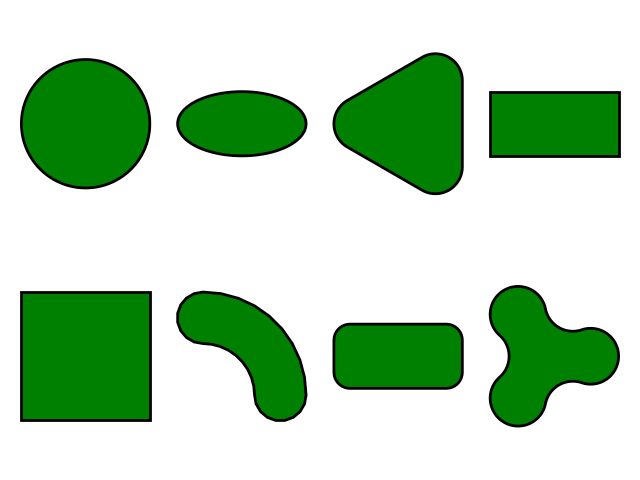
A sample code for plotting various shapes, with default parameters, on the same figure
import gbox as gb
from os import path
import matplotlib.pyplot as plt

fig, axs = plt.subplots(2, 4)
gb.Circle().plot(axis=axs[0, 0])
gb.Ellipse().plot(axis=axs[0, 1])
gb.RegularPolygon(3).plot(axis=axs[0, 2])
gb.Rectangle().plot(axis=axs[0, 3])
gb.BoundingBox2D().plot(axis=axs[1, 0])
gb.CShape().plot(axis=axs[1, 1])
gb.Capsule().plot(axis=axs[1, 2])
gb.NLobeShape(3).plot(axis=axs[1, 3])
plt.tight_layout()
plt.savefig(path.join(path.dirname(__file__), "shapes.pdf"))
plt.close()
It produces the following figure.
Methods#
Points#
Methods for working with points (at present in a plane)
import gbox as gb
from numpy import array, pi

points = gb.Points(array([[2.0, 3.0], [6.0, 6.5], [5.0, 8.0]]))
print(points.x)  # x coordinates of points
print(points.y)  # y coordinates of points
print(len(points))  # 3, i.e., number of points
print(points.dim)  # 2, i.e., the dimensions x and y
points.append(array([[44.0, -5.0], ]), end=True)  # appends points at the end
points.append(array([[44.0, -5.0], ]), end=False)  # appends points at the beginning
points.close_loop()  # appends first point at the end
points.transform(angle=1.5 * pi, dx=-2.5, dy=-4.1)  # rotates points in CCW direction by `angle=1.5 * pi` and
# translates points by `dx` and `dy` along the `x` and `y` directions.
points.reverse()  # reverses the order of points
points.reflect(p1=(0.0, 5.0), p2=(-8.0, 1.0))  # reflects the points about the line joining `p1` and `p2`
Curves#
Methods for working with curves (at present in a plane)
import gbox as gb
from numpy import pi

line = gb.StraightLine(length=1.0, start_point=(2.0, 3.0), angle=pi / 2)
# Creates straight line starting at a given point, of a given length and aligned at an angle with the positive x-axs
line.num_locus_points = 200  # set the number of points along the locus, defaults to 100
print(line.locus)  # points: Points along the locus of the line
#
ell_arc = gb.EllipticalArc(
  smj=2.0, smn=1.0, theta_1=0.25 * pi, theta_2=0.6 * pi, centre=(1.0, -5.0), smj_angle=0.45 * pi
)
# Creates an elliptical arc with specified `centre`, semi major and minor axes of lengths 2.0 and 1.0,
# starting from `theta_1` to `theta_2` (w.r.t semi major axs) and the inclination of semi major axs `smj_angle`.
print(ell_arc.locus)
# points of arc along the locus, default to 100 point which can be set by `ell_arc.num_locus_points`
#
cir_arc = gb.CircularArc(r=2.5, theta_1=0.0 * pi, theta_2=1.25 * pi, centre=(2.0, 4.0))
# Creates a circular arc with radius `r`, starting from `theta_1` and ending at `theta_2`
Closed Shapes#
Methods for working with closed shapes (at present in a plane). For all the shapes the following four common properties are defined
locus:Pointskind of object containing the points along the locus of the shape. The number of points defaults to 100 but can be set to a desired number.area: Enclosed area of the respective shapeperimeter: Perimeter of the respective shapeshape_factor: A non-dimensional number used to quantify the non-circularity of the shape. It is defined as the ratio of the respective shape perimeter to the perimeter of the circle containing equivalent area.
The following snippet shows the various parameters or operations one can do on a closed shape, using the Circle as an example.
import gbox as gb
import matplotlib.pyplot as plt

circle = gb.Circle(radius=2.0, cent=(3.0, 6.0))
print(circle.area)  # prints circle area
print(circle.perimeter)  # prints circle perimeter
print(circle.shape_factor)  # returns shape factor: perimeter/equivalent circle perimeter.
print(circle.locus)  # prints 50 points along the locus of circle
# one can set the desired number of locus points as
circle.num_locus_points = 251
print(circle.locus)  # prints 251 points along the locus of the circle
circle.plot()  # plots a circle displays using `matplotlib.pyplot.show()`
circle.plot(f_path='/path/to/file')  # saves a plot at the specified path
_, axis = plt.subplots()[1]
circle.plot(axis=axis)  # plots circle on the axs object
gb.Rectangle().plot(axis=axis)  # adds rectangle to the same axs
Shapes List#
ShapesList, ClosedShapesList are defined to work efficiently with multiple shapes. For all the closed
shapes list version is available which takes a single numpy array with the respective shape information.
For example,
import gbox as gb
from numpy import array

circles_data = array([
  [0.0, 0.0, 2.0],
  [2.0, 8.0, 3.2],
  [-2.0, 4.0, 1.2],
  [2.0, 4.0, 1.2],
])  # (4, 3) shaped array containing four circles information with first two columns (x, y) coordinates of
# their centres and the last column contains radii.
circles = gb.Circles(circles_data)
circles.plot()  # plots circles on a given axs or to new axs (which can be saved or displayed using plt.show())
print(circles.loci.points.shape)  # (num_circles, num_locus_points, 2) shaped array
print(circles.areas)  # evaluates all circles areas
print(circles.perimeters)  # evaluates all circles perimeters
print(circles.shape_factors)  # evaluates all circles shape_factors